YOLOv1, 2015. One forward pass through a CNN predicts every bounding box and class at once. No region proposals, no sliding window. This is the story of how it got to v10.
Figure: YOLO's single-stage pipeline - one forward pass turns the image into 7×7×30 predictions, then post-processing filters them.
metrics
Metric
Value
Comparison
Speed
45 fps
9× faster than Faster R-CNN
Accuracy
63.4% mAP
-7% vs Faster R-CNN
Grid Size
7×7 cells
49 possible detections
Parameters
~20M
Custom GoogLeNet-inspired backbone (the implementation below uses ResNet34)
Input Size
448×448
Fixed resolution
before YOLO
traditional computer vision
Earlier approaches relied on manually engineered features: HOG (histogram of oriented gradients), SIFT (scale-invariant feature transform), sliding windows across image pyramids. You'd compute pixel gradients, build feature descriptors by hand, and feed them into classifiers like SVMs. The features weren't learned - they were designed by domain experts who understood what edges, textures, and shapes look like.
These hand-built features break down in complex scenes like CCTV footage with:
Dozens of objects
Heavy occlusion
Complex features
Real-time requirements (sliding window detectors run the classifier at every position and scale - expensive)
The feature map encodes what's in the image. Stage 1 proposes where objects might be. Stage 2 refines those proposals and assigns class labels.
The first pass generates proposals (potential object locations), the second refines them into final predictions. This is accurate and each component can be tuned separately, but the multi-stage pipeline is complex, trained piecewise, and far too slow for real-time use (~5 fps on GPU).
comparison: object detection methods (2014-2016)
Method
Year
Speed (fps)
mAP (%)
Pipeline Type
Proposals
Real-time?
R-CNN
2014
0.02
66.0
Two-stage
Selective Search (2000+)
❌
Fast R-CNN
2015
0.5
70.0
Two-stage
Selective Search
❌
Faster R-CNN
2015
7
73.2
Two-stage
RPN (300)
❌
DPM
2015
<1
30.4
Sliding window
Dense sampling
❌
YOLOv1
2016
45
63.4
Single-stage
None
✅
why YOLO: the motivation
The core idea: treat object detection as a single regression problem.
Instead of:
Generate proposals → 2. Classify proposals
Do:
Single network → Box detection + Category prediction simultaneously
One forward pass, one unified loss, and the network sees the whole image at once for global context. That buys real-time speed (45+ fps vs ~5 for two-stage detectors), at the cost of slightly lower accuracy.
Joseph Redmon et al. (2016) built exactly this: one network, one pass, boxes + classes out the other end.
YOLO high level overview
Object detection as a single regression problem:
concept
Input: Image of any size (resized to 448×448)
Process: Divide image into S×S grid cells (S=7 in the paper)
Predict: For each grid cell, predict B bounding boxes and C class probabilities
Output: Tensor of shape S×S×(B×5+C)
why "you only look once"?
Unlike sliding window approaches (like DPM) that run a classifier at every position, or two-stage detectors that process thousands of region proposals, YOLO looks at the image once in a single forward pass.
single pass, end-to-end
No separate proposal generation
No batch processing of regions
One network, one forward pass
Direct prediction from pixels to bounding boxes and classes
Figure: YOLO's single-stage detection pipeline - the entire image is processed once to produce bounding boxes and class predictions
Figure: The complete YOLO detection algorithm from input image to final predictions
the architecture
YOLO is a CNN. 24 convolutional layers for feature extraction, 2 fully connected layers at the end to produce the final output.
Early layers detect low-level stuff (edges, color patches). Deeper layers combine those into higher-level features (eyes, wheels, textures). The FC layers at the end take all of that and produce bounding box predictions.
Backbone (Feature Extraction):
24 convolutional layers with alternating 1×1 and 3×3 filters
4 max-pooling layers for spatial downsampling
Leaky ReLU activation (for all layers except the last)
Convolutions extract spatial features while preserving structure, but simply stacking them doesn't add non-linearity. So between layers you interleave non-linear activations (Leaky ReLU), 1×1 convolutions to cut dimensionality and add non-linearity, and 3×3 convolutions to extract spatial features and downsample.
why leaky ReLU?
Standard ReLU: f(x) = max(0, x) → can cause "dying neurons" (always output 0)
Leaky ReLU: f(x) = x if x > 0 else 0.1*x → allows small negative gradients, preventing dead neurons
regularization techniques:
Dropout (rate=0.5) after the first FC layer
Data augmentation (random scaling, translation, HSV adjustments)
Figure: Complete YOLOv1 network architecture with 24 convolutional layers and 2 fully connected layers
Figure: The full network from input (448×448×3) to output (7×7×30) tensor
how YOLO works
Take the image and lay a grid over it. The original YOLO uses a 7x7 grid. This divides the image into 49 cells.
Each grid cell gets a job. It's responsible for detecting any object whose center point falls within that cell.
Make a prediction for every cell. A single, powerful neural network looks at the whole image and, for every single one of the 49 grid cells, it spits out a prediction. This prediction answers a few key questions:
"Is an object's center in here? How confident am I?"
"If so, where is the bounding box for that object?"
"And what class is it (a dog, a person, a car)?"
That's it. One look, one pass through the network, and out comes a flood of predictions from all 49 cells at once. No proposals, no second stage. Just a direct mapping from image pixels to bounding boxes and class probabilities.
the grid system
Step 1: Divide the 448×448 image into a 7×7 grid (S=7 in the paper)
Each grid cell: 64×64 pixels (448/7 = 64)
Step 2: Assign responsibility
Each cell is responsible for detecting one object
Which object? The one whose center point falls into that cell
Figure: Image divided into 7×7 grid with object center points marked - each cell is responsible for objects whose centers fall within it
Figure: Identifying which grid cell is responsible for each object based on center point location
Figure: Close-up view of how object center points determine grid cell responsibility
Figure: Computing the center point and assigning it to the appropriate grid cell
what does "responsible" mean?
If an object's center point falls into a grid cell, that cell must:
Predict the bounding box coordinates
Predict the confidence that an object is present
Predict the class probabilities
example
Person's center at (100, 200) → falls into grid cell (1, 3)
Horse's center at (300, 150) → falls into grid cell (4, 2)
Grid cell (1, 3) is responsible for detecting "person"
Grid cell (4, 2) is responsible for detecting "horse"
But there's a catch... a big one.
What happens if the center of two objects falls into the same grid cell? Imagine a person standing directly in front of a car.
YOLOv1's limitation: Each grid cell can only detect ONE object.
This is a fundamental rule of the original YOLO. Each cell proposes two bounding boxes (more on that below), but it can only output one set of class probabilities. Two objects in the same cell? Too bad, one gets ignored.
This is YOLOv1's biggest weakness. Crowds, flocks of birds, anything with clustered small objects - it chokes. Later versions fix this. For now: one cell, one vote.
Fixed in YOLOv2+: Anchor boxes allow multiple detections per cell
Impact: Maximum 49 objects per image (7×7 grid). Crowded scenes (flocks of birds, dense crowds) will have missed detections.
bounding box format and encoding
Ground truth bounding box for person: (100, 200, 130, 202)
These are large absolute values
Hard for the network to predict directly
Solution: Make predictions relative to the grid cell
target encoding (ground truth → YOLO format)
For a bounding box with center (x, y), width w, height h:
Figure: 30-dimensional vector format with bounding box coordinates, confidence, and class probabilities
prediction vector
what does each grid cell predict?
Each grid cell outputs a 30-dimensional vector:
Bounding Boxes (B=2 boxes):
Box 1: (x₁', y₁', w₁', h₁', c₁) - 5 values
Box 2: (x₂', y₂', w₂', h₂', c₂) - 5 values
Where:
x', y' = center offset relative to top-left corner of grid cell (0 to 1)
w', h' = width/height relative to entire image (0 to 1)
c = objectness confidence = Pr(Object) × IOU_pred^truth
Class Probabilities (C=20 for Pascal VOC):
[p₁, p₂, ..., p₂₀] - 20 values
These are conditional probabilities: Pr(Class_i | Object)
"What is the probability of each class, given that an object exists in this cell?"
Total: 5×2 + 20 = 30 values per grid cell
For the entire image: 7×7×30 = 1,470 values
why predict 2 boxes per cell?
Objects come in different aspect ratios and sizes, so each cell predicts 2 boxes. During training, each ground truth object is assigned to the box with the highest IOU with it.
At inference: We keep only the box with the highest confidence score for each cell.
understanding confidence score
The confidence c encodes two things:
Pr(Object): Probability that the box contains an object
IOU_pred^truth: How well the predicted box fits the object
text
c = Pr(Object) × IOU_pred^truth
Three scenarios:
No object in cell: c = 0
Object present, poor fit: c = low (e.g., 0.3)
Object present, good fit: c = high (e.g., 0.9)
Figure: How class probabilities are combined with objectness confidence to produce final class-specific confidence scores
Now we have absolute pixel coordinates for the bounding box.
Figure: Converting relative YOLO format coordinates back to absolute pixel coordinates for visualization
step 3: compute class-specific confidence
For each box, multiply objectness by class probabilities:
python
class_confidence = c × max(p₁, p₂, ..., p₂₀)
Example:
Box 1 confidence: c₁ = 0.85
Highest class probability: p₁₄ = 0.9 (person class)
Final confidence: 0.85 × 0.9 = 0.765
step 4: select best box per cell
Each cell predicted 2 boxes → keep the one with highest class-specific confidence.
Example:
Box 1: c₁' = 0.765
Box 2: c₂' = 0.621
Keep Box 1, discard Box 2
Figure: Target confidence values and how they're computed from IOU between predicted and ground truth boxes
step 5: filter by confidence threshold
Remove all boxes with confidence below a threshold (e.g., 0.5):
python
final_boxes = [box for box in boxes if box.confidence > 0.5]
step 6: apply NMS
Many grid cells may detect the same object → use Non-Maximum Suppression to remove duplicates.
post-processing: IOU and NMS
intersection over union (IOU)
What is IOU?
A measure of overlap between two bounding boxes. It tells you how well two boxes align.
Formula:
text
IOU = Area of Intersection / Area of Union
Interpretation:
IOU = 0.0 → No overlap
IOU = 0.5 → Decent overlap
IOU = 0.8+ → Excellent overlap (typically considered a correct detection)
Figure: Intersection over Union (IOU) calculation showing overlap between predicted box (blue) and ground truth box (green), with intersection area highlighted
converting between box formats
Center format: (x_center, y_center, width, height)
Figure: Two common bounding box representations - corner format (x₁,y₁,x₂,y₂) vs center format (x_center, y_center, w, h) and how to convert between them
IOU implementation
python
def iou(pred, gt):
    """
    Calculate Intersection over Union between two bounding boxes.

    Args:
        pred: [x1, y1, x2, y2] predicted box
        gt: [x1, y1, x2, y2] ground truth box

    Returns:
        iou: float between 0 and 1
    """
    pred_x1, pred_y1, pred_x2, pred_y2 = pred
    gt_x1, gt_y1, gt_x2, gt_y2 = gt

    # Find intersection rectangle
    x_topleft = max(pred_x1, gt_x1)
    y_topleft = max(pred_y1, gt_y1)
    x_bottomright = min(pred_x2, gt_x2)
    y_bottomright = min(pred_y2, gt_y2)

    # Check if boxes overlap at all
    if x_bottomright < x_topleft or y_bottomright < y_topleft:
        return 0.0

    # Calculate areas
    intersection = (x_bottomright - x_topleft) * (y_bottomright - y_topleft)
    pred_area = (pred_x2 - pred_x1) * (pred_y2 - pred_y1)
    gt_area = (gt_x2 - gt_x1) * (gt_y2 - gt_y1)
    union = pred_area + gt_area - intersection

    iou = intersection / union
    return iou
non-maximum suppression (NMS)
Multiple grid cells often detect the same object, creating duplicate boxes. NMS keeps only the highest-confidence box and removes the others that significantly overlap with it.
NMS algorithm
For each class separately:
Sort all detections by confidence (descending)
Select the box with highest confidence
Remove all boxes with IOU > threshold (e.g., 0.5) with the selected box
Repeat until no boxes remain
Why per-class? We want to suppress duplicate detections of the same object, but not suppress a person detection because it overlaps with a car detection.
Picking NMS Threshold
Choosing the wrong IOU threshold for NMS drastically affects performance.
Threshold too low (e.g., 0.3):
Suppresses too many boxes
Result: Misses objects that are close together
Example: Two people standing next to each other → only one detected
Threshold too high (e.g., 0.7):
Suppresses too few boxes
Result: Multiple boxes per object (duplicates)
Example: Single person gets 3 bounding boxes
Paper uses 0.5:
Balances duplicate suppression and multi-object detection
Works well for most scenarios
NMS Intuition: Keep the best box, kill everything that overlaps too much with it. Repeat until nothing's left to suppress.
NMS implementation
python
def nms(detections, nms_threshold=0.5):
    """
    Apply Non-Maximum Suppression to remove duplicate detections.

    Args:
        detections: list of [x1, y1, x2, y2, score]
        nms_threshold: IOU threshold for suppression

    Returns:
        keep_detections: filtered list of detections
    """
    # Sort detections by score (descending)
    sorted_det = sorted(detections, key=lambda k: -k[-1])
    keep_detections = []

    while len(sorted_det) > 0:
        # Keep the highest confidence box
        best_box = sorted_det[0]
        keep_detections.append(best_box)

        # Remove this box and all boxes with high overlap
        sorted_det = [
            box for box in sorted_det[1:]
            if iou(best_box[:-1], box[:-1]) < nms_threshold
        ]

    return keep_detections
training process
dataset: Pascal VOC
Pascal VOC 2007 + 2012:
20 object classes
Contains images with bounding box annotations
Standard benchmark for object detection
two-stage training strategy
Why two stages? To help the network learn useful features first, then fine-tune for detection.
stage 1: pretraining (classification)
Task: Image classification on ImageNet
Input size: 224×224
Network: First 20 convolutional layers + 1 FC layer
Goal: Learn general visual features
Why? Reduces training time and improves convergence
stage 2: detection training
Task: Object detection on Pascal VOC
Input size: 448×448 (doubled for finer localization)
Network: Full 24 conv layers + 2 FC layers
Why higher resolution? Detection requires fine-grained spatial information
training hyperparameters
Epochs: ~135 epochs
Batch size: 64
Optimizer: SGD with momentum
Momentum: 0.9
Weight decay: 0.0005
Learning rate schedule:
Epochs 1-5: Warm-up from 10⁻³ to 10⁻² (prevents divergence from unstable gradients)
Epochs 6-75: 10⁻² (main training)
Epochs 76-105: 10⁻³ (fine-tuning)
Epochs 106-135: 10⁻⁴ (final refinement)
Why warm-up? Starting with high learning rate causes unstable gradients and divergence. Gradual warm-up stabilizes training.
data augmentation
To prevent overfitting and improve generalization:
Random scaling and translation: up to 20% of original image size
Random HSV adjustment:
Exposure and saturation: up to 1.5× factor
Helps with lighting variations
Dropout: Rate = 0.5 after first FC layer
annotation format conversion
Original annotation: [x_min, y_min, x_max, y_max, class_id]
Object detection in YOLO is formulated as a regression problem: we're predicting continuous values (box coordinates, confidence scores, class probabilities).
The loss function uses Mean Squared Error (MSE) for all components, but with careful weighting to handle class imbalance and scale differences.
three components of loss
Localization Loss: Ensures predicted box coordinates match ground truth
Confidence Loss: Trains confidence scores to reflect object presence and fit quality
Classification Loss: Ensures correct class probabilities for cells with objects
Total Loss = λ_coord × L_box + L_conf + L_class
the class imbalance problem
Problem: In most images, most grid cells don't contain objects.
~2-5 cells with objects
~44-47 cells without objects
Impact:
Gradients from "no object" cells dominate training
Overwhelms gradients from "object" cells
Network learns to predict "no object" everywhere
Solution: Weight the losses differently
λ_coord = 5: Increase weight of box coordinate loss
λ_noobj = 0.5: Decrease weight of "no object" confidence loss
Intuition: Why λ_coord = 5 and λ_noobj = 0.5?
The Numbers Game:
Typical image: 2-3 cells with objects, 46-47 cells without objects
Ratio: ~20:1 (no-object : object)
Without weighting (all λ = 1):
text
Total confidence loss = 2 × (object conf loss) + 47 × (no-object conf loss)
                     ≈ 2 × 0.5 + 47 × 0.1 = 5.7
                     ≈ 82% from no-object cells!
The "no object" gradient overwhelms "object" gradient → network learns to predict "no object" everywhere.
λ_coord = 5: Emphasizes getting boxes right (5× more important than classification)
λ_noobj = 0.5: De-emphasizes empty cells (2× less important than object cells)
Balance found empirically through ablation studies in the paper
λ_coord=5 says "getting box positions right matters a lot." λ_noobj=0.5 says "empty cells, chill out, you're not that important."
Figure: Visualization of class imbalance problem - most grid cells (gray) contain no objects while only a few (colored) contain objects, showing why we need λ weighting factors
1. localization loss (box regression)
Goal: Make predicted box coordinates close to ground truth.
False Positive (FP): Predicted box doesn't match any ground truth
False Negative (FN): Ground truth object that wasn't detected
precision and recall
With these numbers, we can ask two questions:
Precision: "Of the answers you gave, how many were right?"
Precision = TP / (TP + FP) = 6 / (6 + 2) = 75%
This measures how trustworthy the model's predictions are. A high precision model doesn't make many silly mistakes.
Recall: "Of all the things you should have found, how many did you find?"
Recall = TP / (TP + FN) = 6 / (6 + 4) = 60%
This measures how comprehensive the model is. A high recall model doesn't miss much.
The trade-off
Precision and recall fight each other.
Only predict when you're 100% sure? High precision, low recall. You miss stuff.
Predict aggressively on everything? High recall, low precision. Lots of garbage boxes.
so, what is mAP?
We want both. Average Precision (AP) captures this for a single class - it's the area under the precision-recall curve. Higher AP means the model stays precise even as it tries to find more objects.
Precision-Recall Curve: Plot precision vs recall at different confidence thresholds.
Steps to calculate AP:
Sort all predictions by confidence
For each confidence threshold, compute precision and recall
Plot the curve
Compute area under curve
mAP = average AP across all classes. 20 classes? Compute AP for each, average them.
mAP@0.5: Use IOU threshold of 0.5 to determine TP
mAP@0.75: Use IOU threshold of 0.75 (stricter)
mAP@[0.5:0.95]: Average mAP across IOU thresholds from 0.5 to 0.95 in steps of 0.05
mAP Implementation
python
def compute_map(pred_boxes, gt_boxes, iou_threshold=0.5):
    """
    Calculate mean Average Precision for object detection.

    Args:
        pred_boxes: List of predictions per image
                   [{class: [[x1,y1,x2,y2,score], ...], ...}, ...]
        gt_boxes: List of ground truths per image
                 [{class: [[x1,y1,x2,y2], ...], ...}, ...]
        iou_threshold: IOU threshold to consider a detection as TP

    Returns:
        mean_ap: Mean average precision across all classes
        all_aps: Dictionary of AP for each class
    """
    # Get all class labels from ground truth
    gt_labels = set()
    for im_gt in gt_boxes:
        for cls_key in im_gt.keys():
            gt_labels.add(cls_key)
    gt_labels = sorted(list(gt_labels))

    all_aps = {}
    aps = []

    # Compute AP for each class
    for label in gt_labels:
        # Collect all predictions for this class across all images
        cls_preds = []
        for im_idx, im_pred in enumerate(pred_boxes):
            if label in im_pred:
                for box in im_pred[label]:
                    cls_preds.append((im_idx, box))

        # Sort predictions by confidence (descending)
        cls_preds = sorted(cls_preds, key=lambda k: -k[1][-1])

        # Track which GT boxes have been matched
        gt_matched = [[False for _ in im_gts.get(label, [])]
                      for im_gts in gt_boxes]

        # Count total GT boxes for this class (for recall)
        num_gts = sum([len(im_gts.get(label, [])) for im_gts in gt_boxes])

        # Track TP and FP for each prediction
        tp = [0] * len(cls_preds)
        fp = [0] * len(cls_preds)

        # For each prediction, determine if TP or FP
        for pred_idx, (im_idx, pred_box) in enumerate(cls_preds):
            # Get GT boxes for this image and class
            im_gts = gt_boxes[im_idx].get(label, [])

            # Find best matching GT box
            max_iou_found = -1
            max_iou_gt_idx = -1
            for gt_box_idx, gt_box in enumerate(im_gts):
                gt_box_iou = iou(pred_box[:-1], gt_box)
                if gt_box_iou > max_iou_found:
                    max_iou_found = gt_box_iou
                    max_iou_gt_idx = gt_box_idx

            # TP only if IOU >= threshold AND GT box hasn't been matched yet
            if max_iou_found < iou_threshold or \
               (max_iou_gt_idx >= 0 and gt_matched[im_idx][max_iou_gt_idx]):
                fp[pred_idx] = 1
            else:
                tp[pred_idx] = 1
                gt_matched[im_idx][max_iou_gt_idx] = True

        # Compute cumulative TP and FP
        tp = np.cumsum(tp)
        fp = np.cumsum(fp)

        # Compute precision and recall at each threshold
        recalls = tp / num_gts
        precisions = tp / (tp + fp)

        # Smooth precision curve (ensures precision is monotonic)
        # Add boundary values
        recalls = np.concatenate(([0.0], recalls, [1.0]))
        precisions = np.concatenate(([0.0], precisions, [0.0]))

        # Make precision monotonically decreasing
        for i in range(precisions.size - 1, 0, -1):
            precisions[i - 1] = np.maximum(precisions[i - 1], precisions[i])

        # Compute AP as area under curve
        # Get points where recall changes
        i = np.where(recalls[1:] != recalls[:-1])[0]
        ap = np.sum((recalls[i + 1] - recalls[i]) * precisions[i + 1])

        if num_gts > 0:
            aps.append(ap)
            all_aps[label] = ap
        else:
            all_aps[label] = np.nan

    mean_ap = sum(aps) / len(aps) if len(aps) > 0 else 0.0
    return mean_ap, all_aps
performance and results
speed: real-time detection
YOLOv1 Performance:
45 fps on Nvidia Titan X GPU
155 fps for Fast-YOLO (9 conv layers instead of 24)
This is 9× faster than the previous best (Faster R-CNN at ~5 fps)
Why so fast?
Single forward pass: No region proposals, no batch processing
Unified architecture: One network handles everything
Efficient design: Optimized from the ground up for speed
accuracy comparison
YOLOv1 on Pascal VOC 2007:
mAP: 63.4%
Fast-YOLO: 52.7% mAP
Comparison with other methods:
Faster R-CNN: ~70% mAP, but only 7 fps
DPM (Deformable Part Model): ~30% mAP, slower than YOLO
R-CNN: Higher accuracy, but 47 seconds per image
The trade-off:
YOLO sacrifices ~7% mAP for 9× speed improvement
Enables entirely new applications (real-time video, embedded systems)
key advantages over two-stage detectors
Global reasoning: YOLO sees the entire image during prediction
Understands context (less likely to classify background as object)
Fewer background false positives than Fast R-CNN
Generalization: Better performance on new domains
Learns generalizable features
Better transfer to artwork, sketches, etc.
Simplicity: Single network, end-to-end training
No separate proposal generation
Unified loss function
Easier to optimize
Real-time performance: 45+ fps enables:
Live video analysis
Robotics and autonomous vehicles
Interactive applications
Figure: Performance comparison of YOLOv1 with other detection methods on Pascal VOC 2007 dataset
Figure: Detailed accuracy and speed metrics showing YOLO's superiority in real-time performance while maintaining competitive accuracy
limitations of YOLOv1
YOLOv1 trades accuracy for speed, and the trade shows up in a few specific places.
One object per cell. Each cell predicts 2 boxes but only one set of class probabilities, so it detects at most 49 objects (7×7) and breaks on crowds: flocks of birds, dense crowds, or a dog and a bicycle whose centers land in the same cell. One of them gets missed.
Small objects. The 7×7 grid is coarse (each cell ≈ 64×64 px), so small objects barely activate any cell, and groups of them collide in one cell.
Unusual aspect ratios. The network learns aspect-ratio priors from the training data, so long, thin, or oddly shaped objects (a limousine, a tall narrow doorway) get missed.
Localization. A coarse 7×7 feature map and no iterative refinement (unlike Faster R-CNN) mean looser boxes, which hurts mAP at higher IOU thresholds.
Box-size sensitivity. Even with √w and √h, MSE doesn't perfectly balance small vs large box errors.
Class imbalance. Even with λ_noobj = 0.5, the ~20× more "no object" cells push confidence scores systematically lower, so hard objects still get missed.
evolution: from v1 to v10
the YOLO family tree
Each version after v1 tried to fix its problems without killing the speed.
key improvements across versions
YOLOv2 (YOLO9000) - 2017:
Anchor boxes: Instead of predicting boxes directly, predict offsets from predefined anchors
Batch normalization: Added to all conv layers, improved convergence
High-resolution classifier: Pretrain at 448×448 (not 224×224)
Multi-scale training: Train on different input sizes
Binary classification: Use logistic regression instead of softmax (allows multi-label)
Performance: 57.9% mAP@0.5, comparable to RetinaNet but 3-4× faster
YOLOv4 - 2020:
Bag of freebies: Techniques that improve accuracy without increasing inference cost
Data augmentation (Mosaic, MixUp)
Label smoothing
DropBlock regularization
Bag of specials: Techniques with small inference cost increase
Mish activation
CSPNet backbone
SPP (Spatial Pyramid Pooling)
PANet neck
Performance: 43.5% mAP@0.5:0.95, the best at the time
YOLOv5 - 2020 (Ultralytics):
PyTorch implementation: Easier to use and customize
Auto-learning anchors: Automatically cluster anchors from training data
Model family: Nano, Small, Medium, Large, XLarge variants
Better augmentations: Albumentations integration
Export options: ONNX, TensorRT, CoreML, etc.
YOLOv6, v7, v8 (2022-2023): Mostly incremental improvements. v6 (Meituan) focused on industrial deployment with a hardware-aware design. v7 introduced re-parameterized convolutions and a more efficient training pipeline. v8 (Ultralytics) went anchor-free and decoupled the classification and regression heads. All three pushed accuracy up a few points on COCO, but the next real architectural jump is v10.
YOLOv10 - 2024:
NMS-free detection: Eliminates need for NMS post-processing
Consistent matching strategy during training
Dual label assignment
Significantly faster inference
Efficiency optimizations:
Compact inverted block design
Partial self-attention
Spatial-channel decoupled downsampling
Model variants: N/S/M/B/L/X for different speed/accuracy trade-offs
Performance:
YOLOv10-X: ~54% mAP@0.5:0.95 on COCO
YOLOv10-N: Real-time on edge devices
key shifts across versions
v1→v2: Direct prediction → Anchor-based
v2→v3: Single-scale → Multi-scale detection
v3→v4: Manual design → Automated architecture search and bag-of-tricks
Single-stage detection: One network, one forward pass
Real-time performance: Speed is a primary goal
End-to-end training: Unified loss function
Practical focus: Easy to deploy and use
YOLOv10: what's actually new
Two things that actually matter in v10: NMS-free detection and a rethought architecture.
1. NMS-free training with dual heads
Traditional YOLO models generate multiple overlapping boxes per object, then rely on Non-Maximum Suppression (NMS) as post-processing. NMS adds latency and isn't differentiable, so you can't optimize it end-to-end. YOLOv10 gets rid of it entirely.
The trick is two detection heads during training:
One-to-Many (o2m) Head: Matches each ground truth object with multiple predictions. Rich supervision signal - explores diverse locations for the same object.
One-to-One (o2o) Head: Matches each ground truth object with exactly one prediction. Learns to output one clean box per object.
Both heads share the same matching metric so their supervision stays consistent. During training, the o2o head benefits from the rich signal of the o2m head (which explores multiple locations) while learning to produce clean, single predictions. At inference, the o2m head is discarded entirely - zero extra cost. You just use the o2o head, pick top-K class scores, filter by confidence, and you're done. No NMS needed.
The result: about 40% faster inference than YOLOv8 since there's no post-processing overhead, and cleaner predictions with one strong box per object.
2. architectural efficiency
YOLOv10 also rethinks the model architecture for better speed-accuracy tradeoffs:
Lightweight classification head: The classification head in YOLOv8 was 2.5x heavier than the regression head despite regression being more important for accuracy. YOLOv10 replaces it with depthwise separable convolutions - much cheaper.
Decoupled downsampling: Instead of one expensive 3x3 stride-2 conv that handles both spatial reduction and channel expansion, YOLOv10 splits it into a pointwise conv (channels) and a depthwise conv (spatial). Significantly cheaper.
Rank-guided block design: Not all network stages are equally important. YOLOv10 computes the intrinsic rank of each stage's convolutions (via SVD), then replaces redundant stages with lightweight Compact Inverted Blocks while keeping high-rank stages strong with large kernel convolutions and Partial Self-Attention.
comparison: YOLOv1 vs YOLOv10
Caveat: the two columns use different datasets (VOC for v1, a custom object-detection set for v10), so read the mAP jump as directional, not like-for-like. On COCO, YOLOv10 reports ~54% mAP50-95.
Metric
YOLOv1 (2016)
YOLOv10 (2024)
mAP50
63.4% (VOC)
90.6% (ODN dataset)
mAP50-95
Not reported
76%
Speed (fps)
45 fps
~63 fps (40% faster than v8)
Grid Size
7×7 (fixed)
Multi-scale, adaptive
Boxes per Cell
2
Dynamic (o2o/o2m)
Max Objects
49 (7×7 grid limit)
Unlimited
Post-processing
NMS required
NMS-free
Small Objects
Struggles
Excellent (multi-scale detection)
Architecture
24 conv + 2 FC
Efficient CSPNet + lightweight heads
Training
Single-head
Dual-head (o2m + o2o)
v1 proved single-stage detection works. v10 makes it truly end-to-end - no post-processing, even faster. Same core idea, just way more refined.
implementation: PyTorch code examples
Full PyTorch implementation of YOLOv1 below.
1. model architecture
The YOLO network uses a ResNet34 backbone (pretrained on ImageNet) followed by detection layers:
python
import torchimport torch.nn as nnimport torchvisionclass YOLOV1(nn.Module): """ YOLOv1 Implementation using ResNet34 backbone Args: img_size: Input image size (448x448) num_classes: Number of classes (20 for Pascal VOC) model_config: Configuration dict with S, B, and architectural params Output: Tensor of shape (batch_size, S, S, 5*B + C) """ def __init__(self, img_size, num_classes, model_config): super(YOLOV1, self).__init__() self.img_size = img_size self.S = model_config['S'] # Grid size (7x7) self.B = model_config['B'] # Boxes per cell (2) self.C = num_classes # Number of classes (20) # Load pretrained ResNet34 backbone (trained on ImageNet 224x224) backbone = torchvision.models.resnet34( weights=torchvision.models.ResNet34_Weights.IMAGENET1K_V1 ) # Feature extraction layers (before FC layers) self.features = nn.Sequential( backbone.conv1, # 7x7 conv, stride 2 backbone.bn1, backbone.relu, backbone.maxpool, backbone.layer1, # ResNet blocks backbone.layer2, backbone.layer3, backbone.layer4, # Output: 512 channels ) # Detection head: 3 conv layers for feature refinement yolo_conv_channels = model_config['yolo_conv_channels'] # 1024 leaky_relu_slope = model_config['leaky_relu_slope'] # 0.1 self.conv_layers = nn.Sequential( nn.Conv2d(512, yolo_conv_channels, 3, padding=1, bias=False), nn.BatchNorm2d(yolo_conv_channels), nn.LeakyReLU(leaky_relu_slope), nn.Conv2d(yolo_conv_channels, yolo_conv_channels, 3, stride=2, padding=1, bias=False), nn.BatchNorm2d(yolo_conv_channels), nn.LeakyReLU(leaky_relu_slope), nn.Conv2d(yolo_conv_channels, yolo_conv_channels, 3, padding=1, bias=False), nn.BatchNorm2d(yolo_conv_channels), nn.LeakyReLU(leaky_relu_slope) ) # Final 1x1 conv to get S*S*(5B+C) output self.final_conv = nn.Conv2d(yolo_conv_channels, 5 * self.B + self.C, 1) def forward(self, x): # x: (batch, 3, 448, 448) out = self.features(x) # (batch, 512, 14, 14) out = self.conv_layers(out) # (batch, 1024, 7, 7) out = self.final_conv(out) # (batch, 30, 7, 7) # Permute to (batch, S, S, 5B+C) out = out.permute(0, 2, 3, 1) # (batch, 7, 7, 30) return out
2. loss function
The complete YOLOv1 loss with all three components:
import torchimport albumentations as albimport cv2from torch.utils.data import Datasetclass VOCDataset(Dataset): """Pascal VOC Dataset with YOLO target encoding""" def __init__(self, split='train', img_size=448, S=7, B=2, C=20): self.split = split self.img_size = img_size self.S = S # Grid size self.B = B # Boxes per cell self.C = C # Number of classes # Data augmentation for training self.transforms = { 'train': alb.Compose([ alb.HorizontalFlip(p=0.5), alb.Affine(scale=(0.8, 1.2), translate_percent=(-0.2, 0.2)), alb.ColorJitter(brightness=(0.8, 1.2), saturation=(0.8, 1.2)), alb.Resize(self.img_size, self.img_size) ], bbox_params=alb.BboxParams(format='pascal_voc', label_fields=['labels'])), 'test': alb.Compose([ alb.Resize(self.img_size, self.img_size) ], bbox_params=alb.BboxParams(format='pascal_voc', label_fields=['labels'])) } # Load Pascal VOC annotations... # (XML parsing code omitted for brevity) def __getitem__(self, index): # Load image and annotations img_info = self.images_info[index] img = cv2.imread(img_info['filename']) img = cv2.cvtColor(img, cv2.COLOR_BGR2RGB) bboxes = [det['bbox'] for det in img_info['detections']] # (x1,y1,x2,y2) labels = [det['label'] for det in img_info['detections']] # Apply augmentations transformed = self.transforms[self.split]( image=img, bboxes=bboxes, labels=labels ) img = transformed['image'] bboxes = torch.tensor(transformed['bboxes']) labels = torch.tensor(transformed['labels']) # Normalize image to [0, 1] and apply ImageNet normalization img_tensor = torch.from_numpy(img / 255.0).permute(2, 0, 1).float() # --- Create YOLO target tensor --- target_dim = 5 * self.B + self.C yolo_target = torch.zeros(self.S, self.S, target_dim) h, w = img.shape[:2] cell_size = h // self.S # Pixels per grid cell if len(bboxes) > 0: # Convert (x1, y1, x2, y2) → (x_center, y_center, width, height) box_width = bboxes[:, 2] - bboxes[:, 0] box_height = bboxes[:, 3] - bboxes[:, 1] box_center_x = bboxes[:, 0] + 0.5 * box_width box_center_y = bboxes[:, 1] + 0.5 * box_height # Determine which grid cell each object belongs to grid_i = torch.floor(box_center_x / cell_size).long() grid_j = torch.floor(box_center_y / cell_size).long() # Compute relative coordinates within grid cell (0 to 1) box_x_offset = (box_center_x - grid_i * cell_size) / cell_size box_y_offset = (box_center_y - grid_j * cell_size) / cell_size # Normalize width and height to image size box_w_norm = box_width / w box_h_norm = box_height / h # Fill YOLO target tensor for idx in range(len(bboxes)): # Assign same target to all B boxes (model picks responsible one) for b in range(self.B): s = 5 * b yolo_target[grid_j[idx], grid_i[idx], s] = box_x_offset[idx] yolo_target[grid_j[idx], grid_i[idx], s+1] = box_y_offset[idx] yolo_target[grid_j[idx], grid_i[idx], s+2] = box_w_norm[idx].sqrt() yolo_target[grid_j[idx], grid_i[idx], s+3] = box_h_norm[idx].sqrt() yolo_target[grid_j[idx], grid_i[idx], s+4] = 1.0 # Confidence # One-hot encode class label = int(labels[idx]) yolo_target[grid_j[idx], grid_i[idx], 5*self.B + label] = 1.0 return img_tensor, yolo_target
4. training loop
Training loop:
python
import torchfrom torch.optim import SGDfrom torch.optim.lr_scheduler import MultiStepLRfrom torch.utils.data import DataLoader# Initialize model, loss, and datasetdevice = torch.device('cuda' if torch.cuda.is_available() else 'cpu')model = YOLOV1(img_size=448, num_classes=20, model_config={ 'S': 7, 'B': 2, 'yolo_conv_channels': 1024, 'leaky_relu_slope': 0.1}).to(device)criterion = YOLOLoss(S=7, B=2, C=20)train_dataset = VOCDataset(split='train', img_size=448)train_loader = DataLoader(train_dataset, batch_size=64, shuffle=True)# Optimizer: SGD with momentum (as per paper)optimizer = SGD(model.parameters(), lr=0.001, momentum=0.9, weight_decay=5e-4)# Learning rate schedule: reduce at epochs [75, 105]# Paper uses warm-up from 1e-3 to 1e-2 for first epochs, then steps downscheduler = MultiStepLR(optimizer, milestones=[75, 105], gamma=0.1)# Training loopnum_epochs = 135 # As per papermodel.train()for epoch in range(num_epochs): epoch_loss = 0.0 for images, targets in train_loader: images = images.to(device) targets = targets.to(device) # Forward pass predictions = model(images) loss = criterion(predictions, targets) # Backward pass optimizer.zero_grad() loss.backward() optimizer.step() epoch_loss += loss.item() scheduler.step() print(f'Epoch {epoch+1}/{num_epochs}, Loss: {epoch_loss/len(train_loader):.4f}')
5. inference with NMS
Converting raw predictions to actual boxes:
python
def convert_predictions_to_boxes(predictions, S=7, B=2, C=20, conf_threshold=0.2, nms_threshold=0.5): """ Convert YOLO predictions to bounding boxes with NMS. Args: predictions: (S, S, 5*B + C) tensor conf_threshold: Minimum confidence to keep box nms_threshold: IOU threshold for NMS Returns: boxes: (N, 4) tensor in (x1, y1, x2, y2) format scores: (N,) confidence scores labels: (N,) class labels """ predictions = predictions.reshape(S, S, 5*B + C) # Get class predictions (same for all boxes in a cell) class_probs, class_labels = predictions[..., 5*B:].max(dim=-1) # Create coordinate shift grid shifts_x = torch.arange(S, device=predictions.device) / float(S) shifts_y = torch.arange(S, device=predictions.device) / float(S) shifts_y, shifts_x = torch.meshgrid(shifts_y, shifts_x, indexing='ij') all_boxes = [] all_scores = [] all_labels = [] # Process each of B boxes per cell for b in range(B): # Extract box parameters x_offset = predictions[..., b*5 + 0] y_offset = predictions[..., b*5 + 1] w = predictions[..., b*5 + 2] h = predictions[..., b*5 + 3] conf = predictions[..., b*5 + 4] # Convert to absolute coordinates x_center = (x_offset / S + shifts_x) y_center = (y_offset / S + shifts_y) width = torch.square(w) # w = √w_pred² height = torch.square(h) # Convert to (x1, y1, x2, y2) format x1 = (x_center - 0.5 * width).reshape(-1, 1) y1 = (y_center - 0.5 * height).reshape(-1, 1) x2 = (x_center + 0.5 * width).reshape(-1, 1) y2 = (y_center + 0.5 * height).reshape(-1, 1) boxes = torch.cat([x1, y1, x2, y2], dim=-1) # Compute class-specific confidence scores scores = conf.reshape(-1) * class_probs.reshape(-1) labels = class_labels.reshape(-1) all_boxes.append(boxes) all_scores.append(scores) all_labels.append(labels) # Concatenate all boxes boxes = torch.cat(all_boxes, dim=0) scores = torch.cat(all_scores, dim=0) labels = torch.cat(all_labels, dim=0) # Confidence thresholding keep = scores > conf_threshold boxes = boxes[keep] scores = scores[keep] labels = labels[keep] # Apply NMS per class keep_mask = torch.zeros_like(scores, dtype=torch.bool) for class_id in torch.unique(labels): class_indices = labels == class_id class_boxes = boxes[class_indices] class_scores = scores[class_indices] # NMS (using torchvision) keep_indices = torch.ops.torchvision.nms( class_boxes, class_scores, nms_threshold ) # Mark these boxes as kept class_keep_indices = torch.where(class_indices)[0][keep_indices] keep_mask[class_keep_indices] = True final_boxes = boxes[keep_mask] final_scores = scores[keep_mask] final_labels = labels[keep_mask] return final_boxes, final_scores, final_labels# Example usagemodel.eval()with torch.no_grad(): img_tensor = ... # Load and preprocess image predictions = model(img_tensor.unsqueeze(0))[0] # Remove batch dim boxes, scores, labels = convert_predictions_to_boxes( predictions, conf_threshold=0.2, nms_threshold=0.5 ) # boxes: (N, 4) in normalized 0-1 coordinates # Multiply by image dimensions to get pixel coordinates
key implementation details
√w and √h: The model predicts square root of width/height to balance loss across different box sizes
Relative Coordinates: x,y offsets are relative to grid cell top-left corner
Responsible Box Selection: During training, only the box with highest IOU with GT is penalized for coordinates
Class Probabilities: Shared across all B boxes in a cell (limitation of v1)
Lambda Weighting: λ_coord=5 to emphasize localization, λ_noobj=0.5 to de-emphasize empty cells
Follows the original paper. Gets ~63% mAP on Pascal VOC 2007 after 135 epochs.
deploying for speed
The usual production path: export to ONNX, then TensorRT, and drop precision. FP16 roughly doubles throughput at near-baseline accuracy; INT8 quantization (quantization-aware training keeps accuracy highest) shrinks the model ~4x for edge devices like Jetson. TensorRT also fuses Conv → BatchNorm → ReLU into single kernels and reuses memory buffers across layers.
The core insight from 2016: treat detection as a single regression problem instead of a multi-stage pipeline. Ten versions later, the models are faster and more accurate, but that basic idea hasn't changed.
references
Redmon, J., Divvala, S., Girshick, R., & Farhadi, A. (2016). You Only Look Once: Unified, Real-Time Object Detection. CVPR 2016.
Get predictions: bboxes (x,y,w,h), class probabilities, objectness scores
Network has ~20M parameters (backbone + neck + head)
c. Loss Calculation
Box loss (7.5x weight): IoU/GIoU loss for bbox coordinates
Class loss (1.5x weight): Binary cross-entropy for classification
DFL loss (1.5x weight): Distribution focal loss for bbox refinement
Total loss = weighted sum of above
What do these mean?
Box loss: How well the model draws a box around the phone
Class loss: How sure the model is that the thing is a phone
DFL loss: How precisely the model guesses the edges of the box
d. Backward Pass
Calculate gradients using total loss
Backpropagation and updating of gradients using Optimizer (I used AdamW with momentum)
e. Optimizer Step (AdamW)
Update weights using gradients
Apply learning rate (starts at 0.0005, decays to 0.01 × lr0)
Apply weight decay (0.0005) for regularization
Apply momentum (0.9)
2. validation (every epoch)
After all training batches:
a. Switch to eval mode
Disable dropout (full model instead of skipping some layers)
Use batch normalization in eval mode (already learned features instead of learning new ones)
No augmentations (no flips)
b. For each validation image
Forward pass (no gradient calculation)
Get predictions with conf threshold (default 0.001 for val)
Apply NMS (non-maximum suppression: if the model draws many boxes on the same phone, keep only the best one and throw away the rest) with IoU threshold 0.45
c. Metric Calculation
Match predictions to ground truth (IoU >= 0.5)
Calculate per-class metrics:
Precision = TP / (TP + FP)
Recall = TP / (TP + FN)
mAP@50 = mean AP at IoU=0.5
mAP@50-95 = mean AP averaged over IoU 0.5 to 0.95
Calculate overall metrics (averaged across all classes)
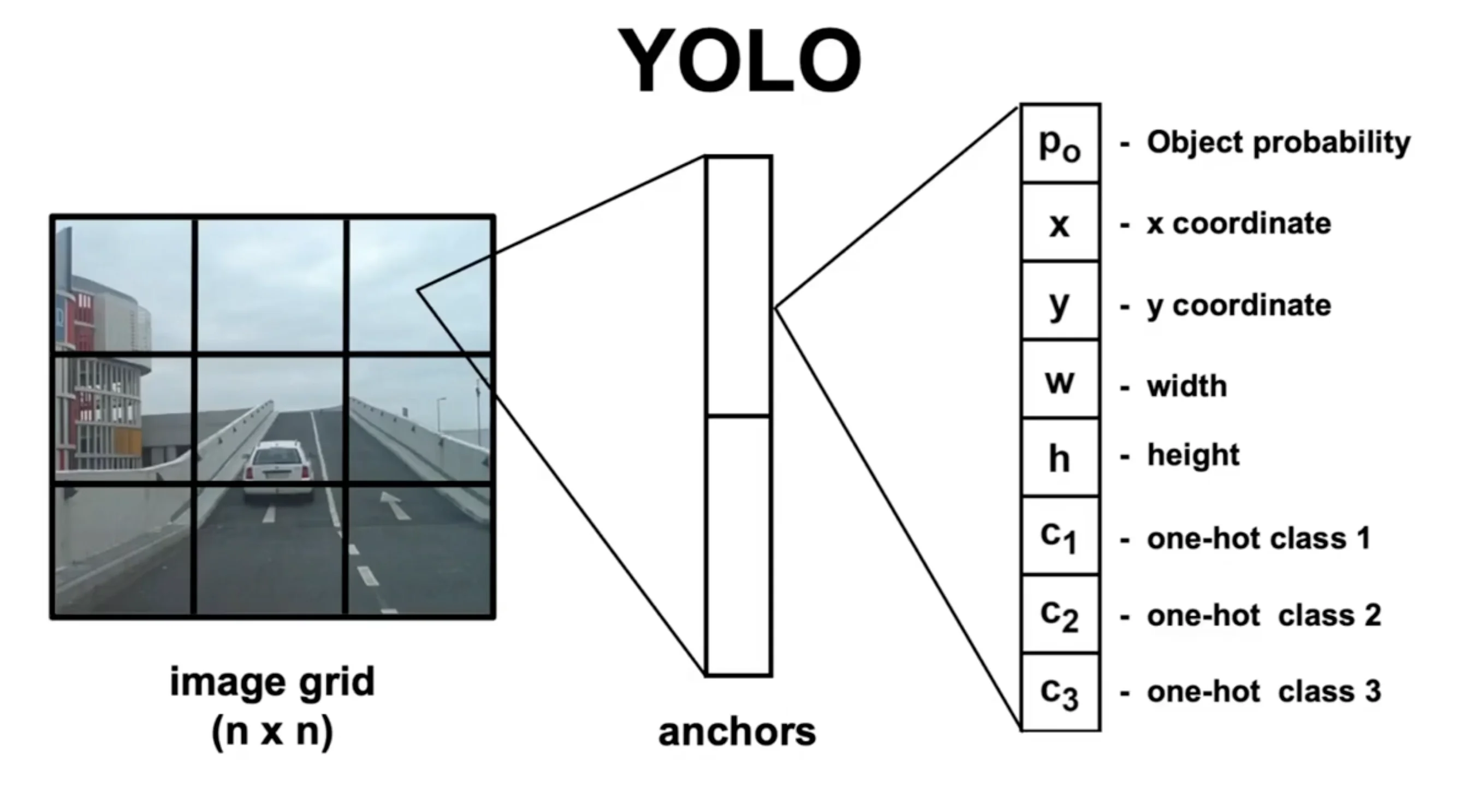 Figure: YOLO's single-stage detection pipeline - the entire image is processed once to produce bounding boxes and class predictions
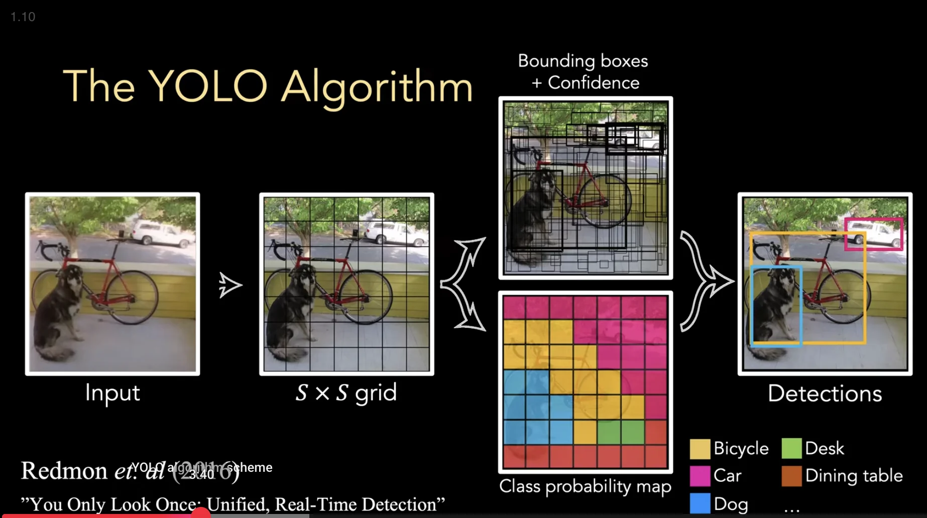 Figure: The complete YOLO detection algorithm from input image to final predictions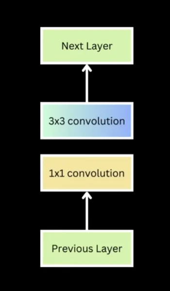
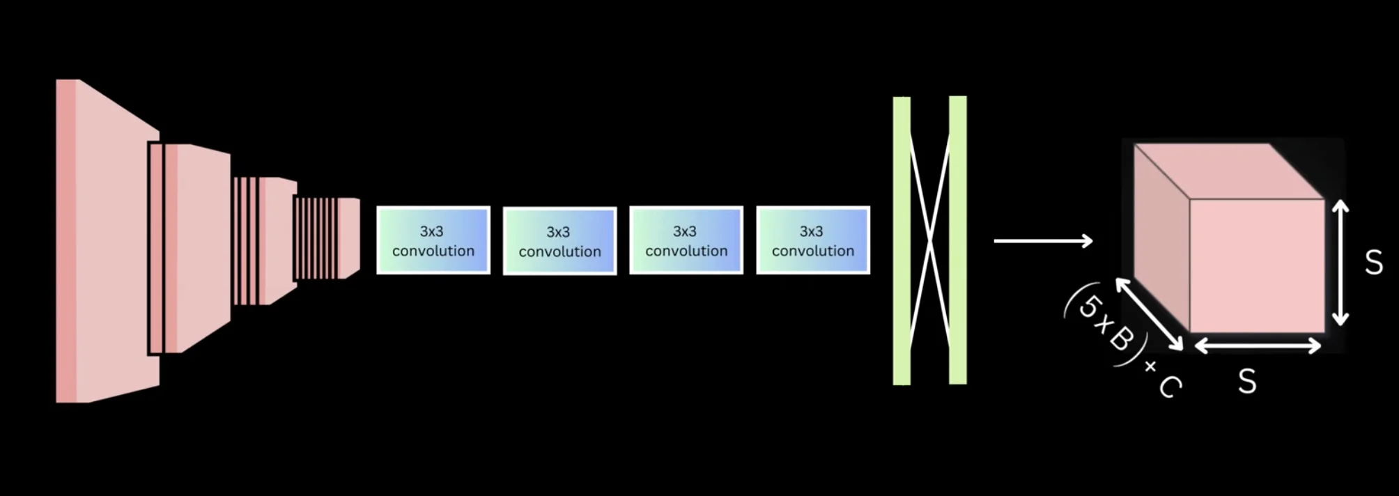
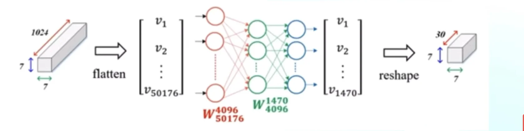
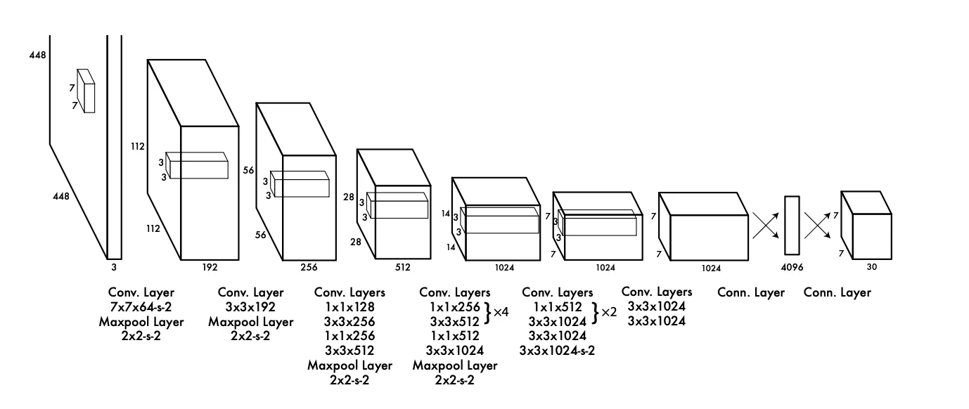 Figure: Complete YOLOv1 network architecture with 24 convolutional layers and 2 fully connected layers
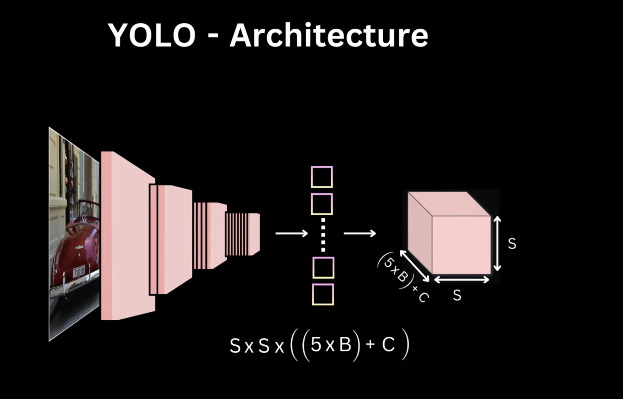 Figure: Layer-by-layer breakdown showing filter sizes, dimensions, and feature map transformations
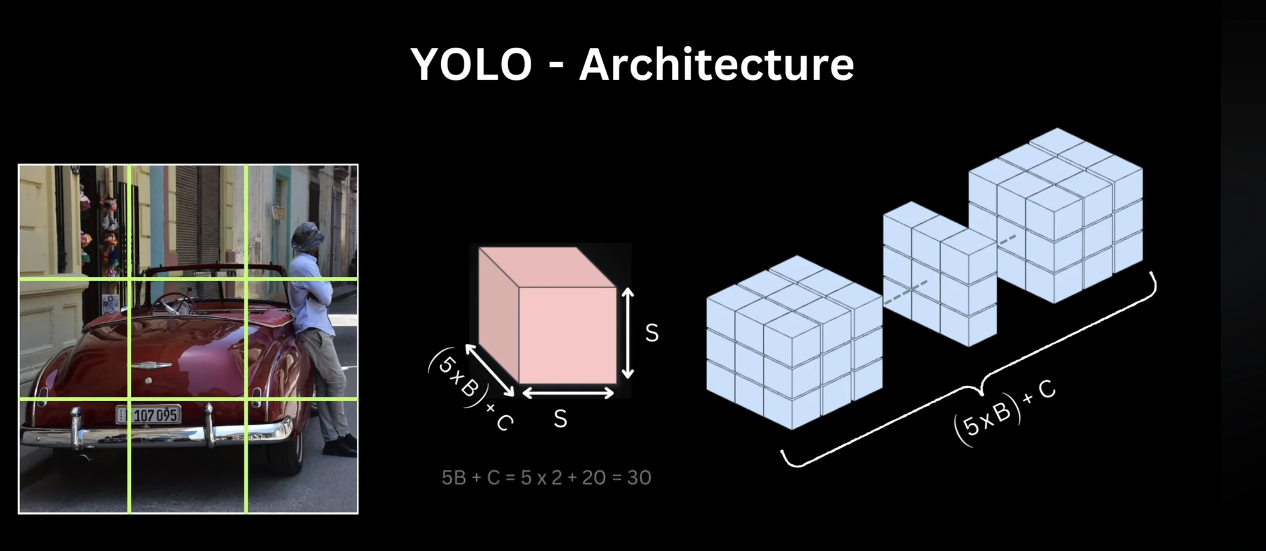 Figure: The full network from input (448×448×3) to output (7×7×30) tensor
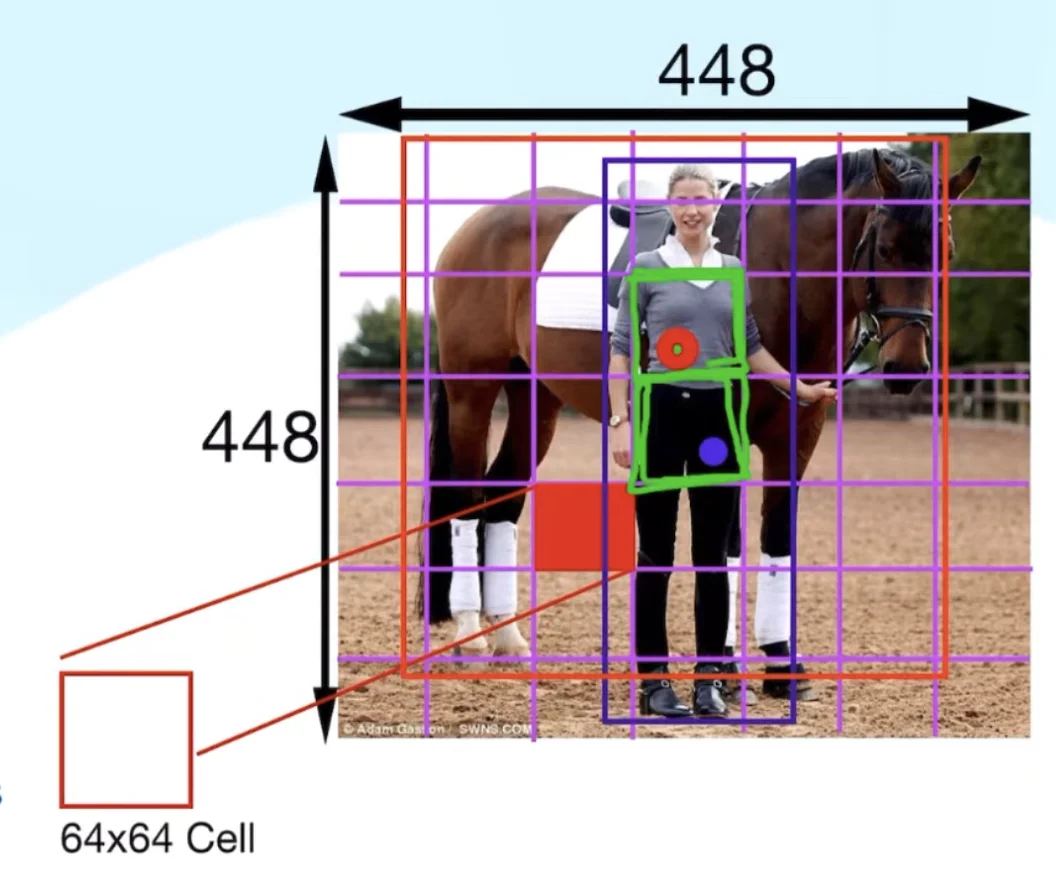 Figure: Image divided into 7×7 grid with object center points marked - each cell is responsible for objects whose centers fall within it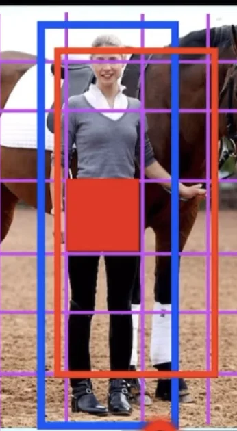
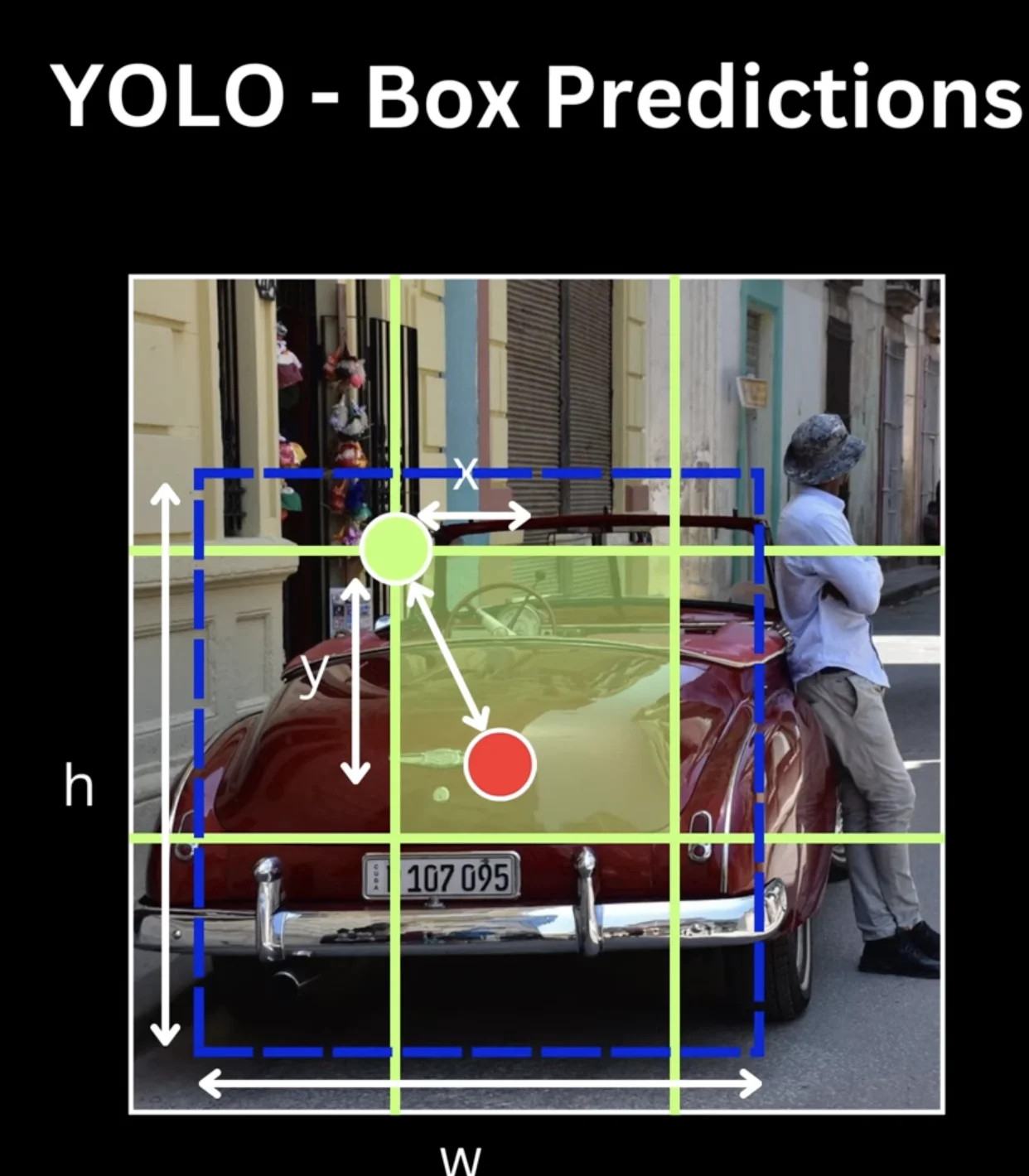 Figure: Close-up view of how object center points determine grid cell responsibility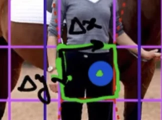
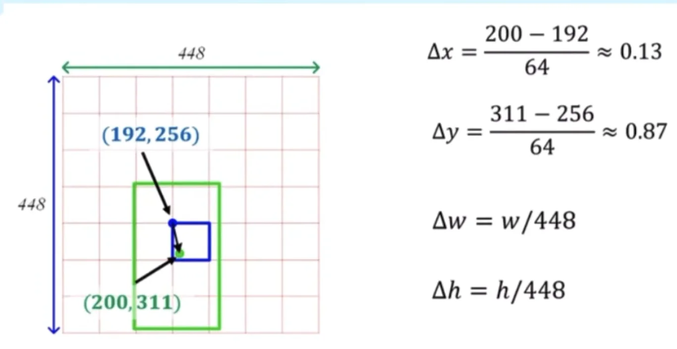 Figure: Computing relative offsets (Δx, Δy) from grid cell top-left corner to object center
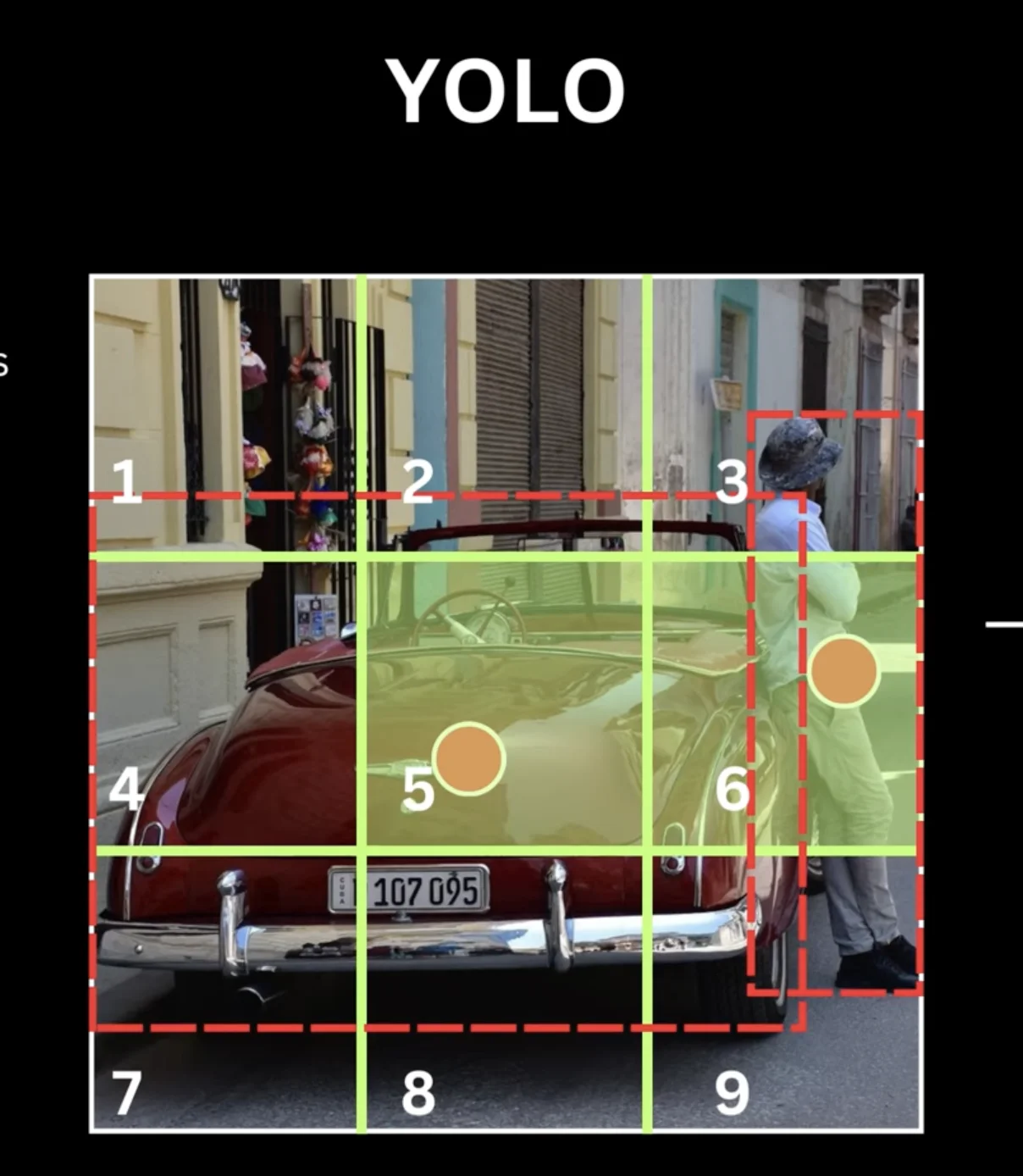 Figure: Detailed breakdown of how center coordinates are normalized relative to grid cell dimensions
 Figure: Visualizing the x,y center point encoding process with actual coordinate values
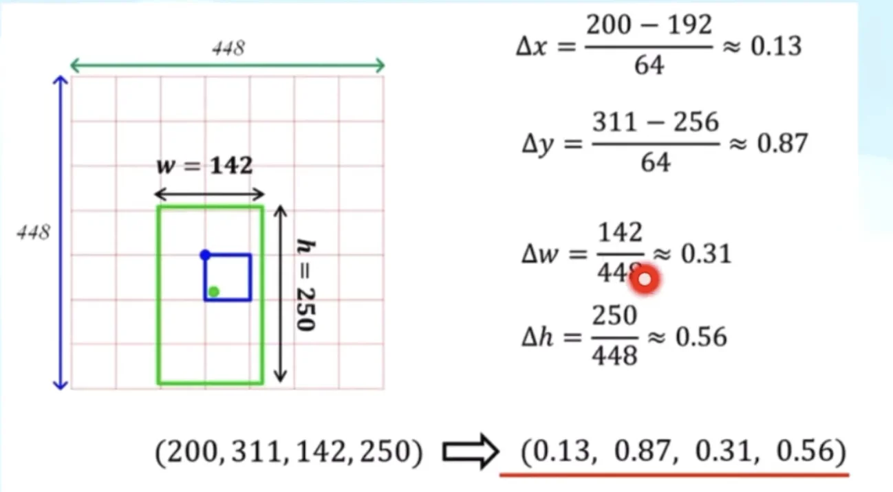 Figure: Final normalized ground truth values (x', y', w', h') ready for training
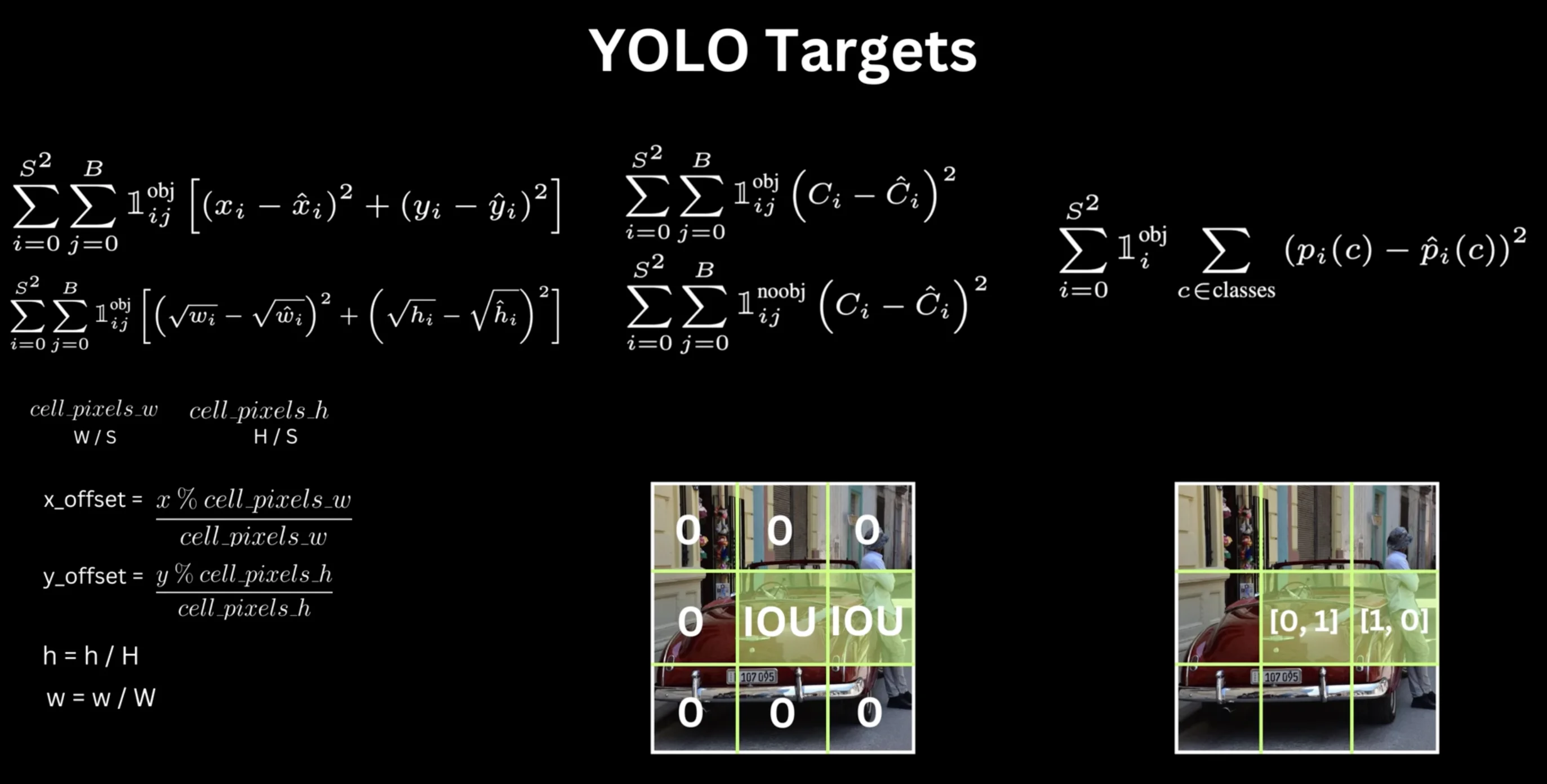 Figure: 30-dimensional vector format with bounding box coordinates, confidence, and class probabilities
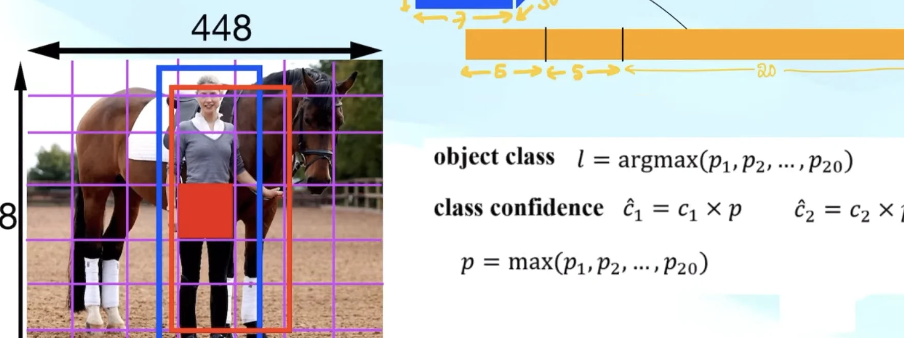 Figure: How class probabilities are combined with objectness confidence to produce final class-specific confidence scores
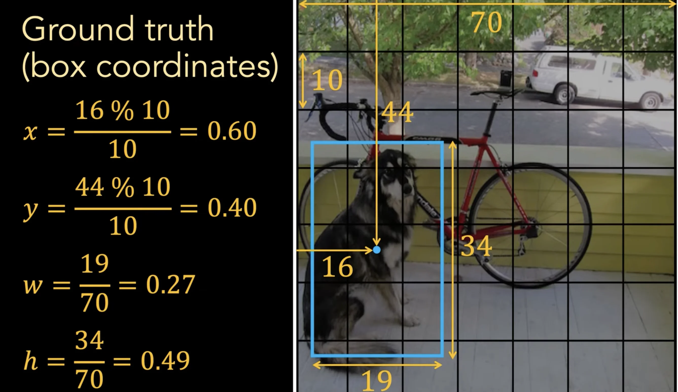 Figure: Converting relative YOLO format coordinates back to absolute pixel coordinates for visualization
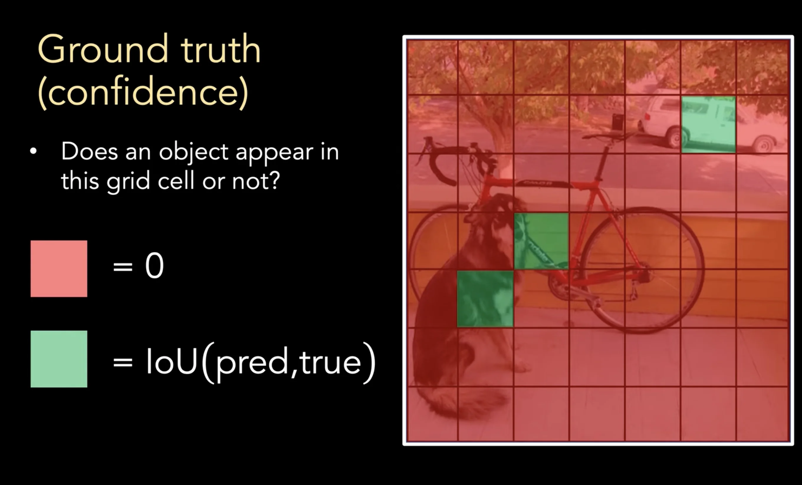 Figure: Target confidence values and how they're computed from IOU between predicted and ground truth boxes
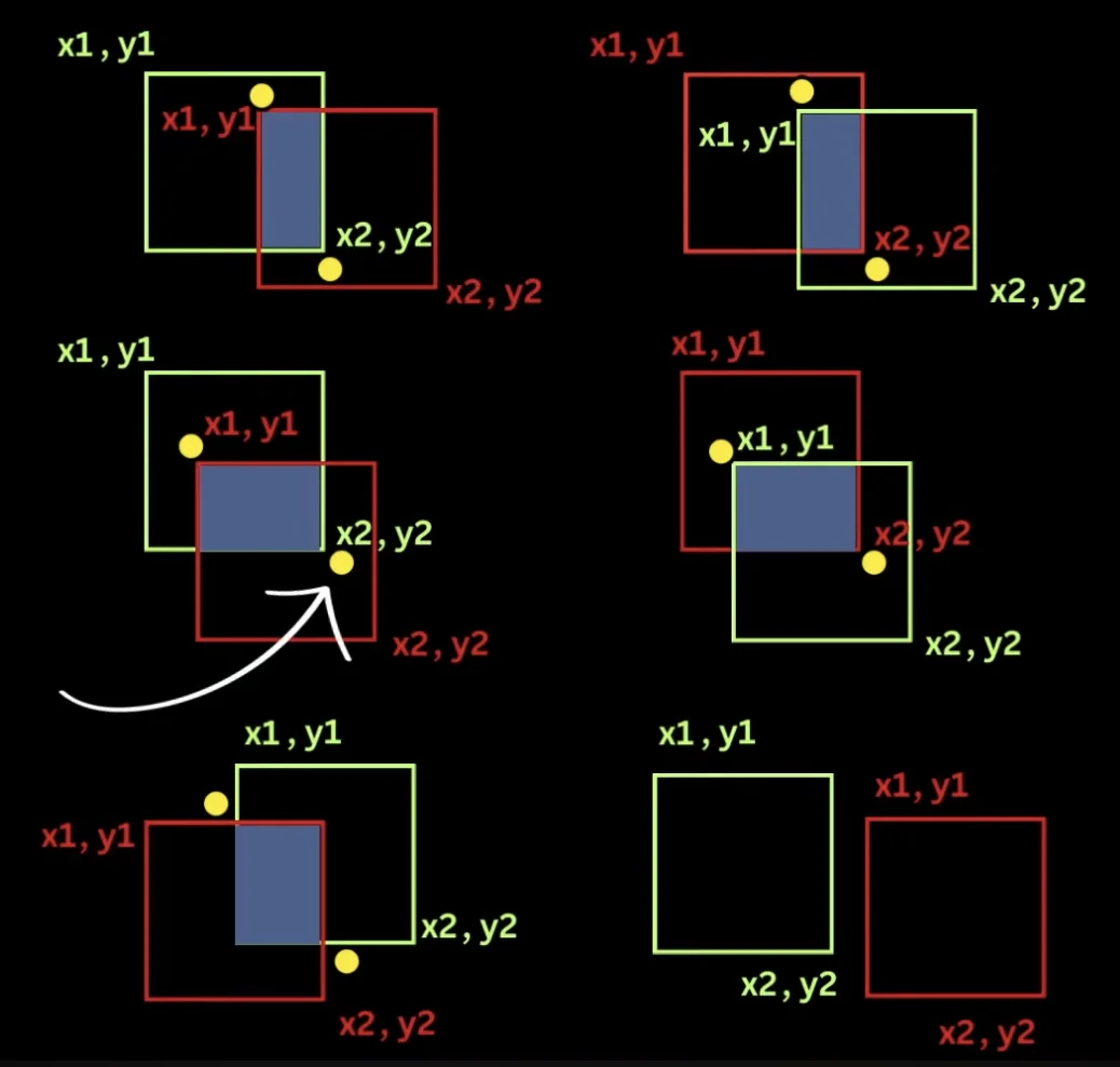 Figure: Intersection over Union (IOU) calculation showing overlap between predicted box (blue) and ground truth box (green), with intersection area highlighted
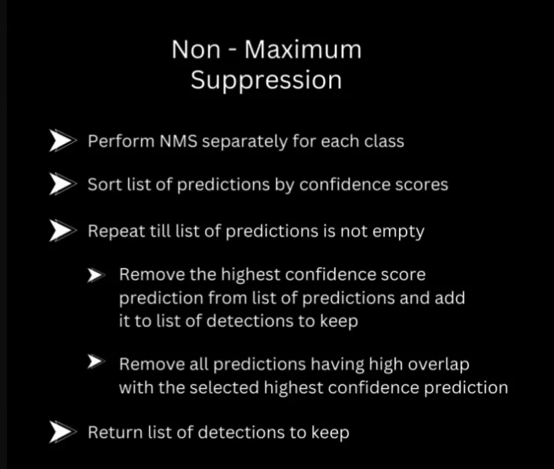
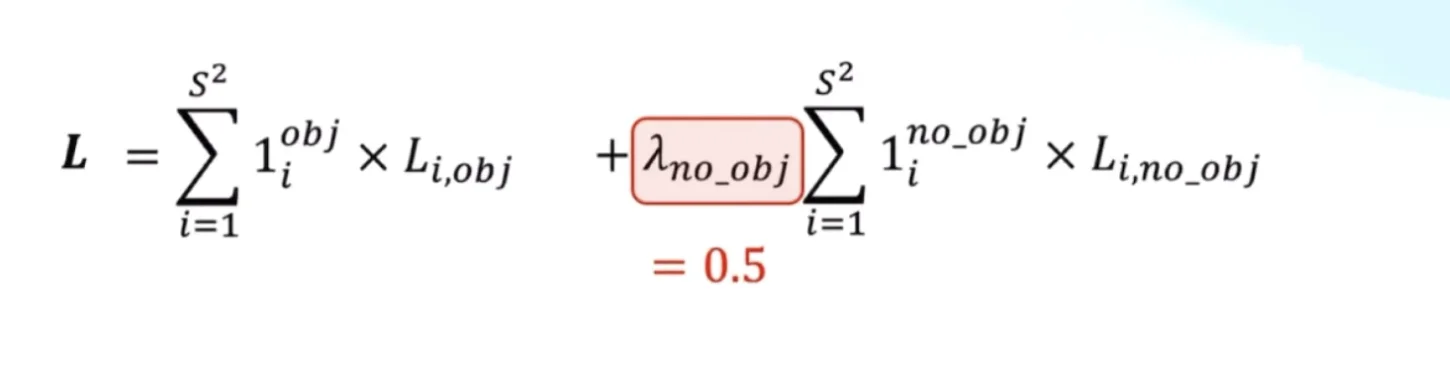 Figure: Visualization of class imbalance problem - most grid cells (gray) contain no objects while only a few (colored) contain objects, showing why we need λ weighting factors
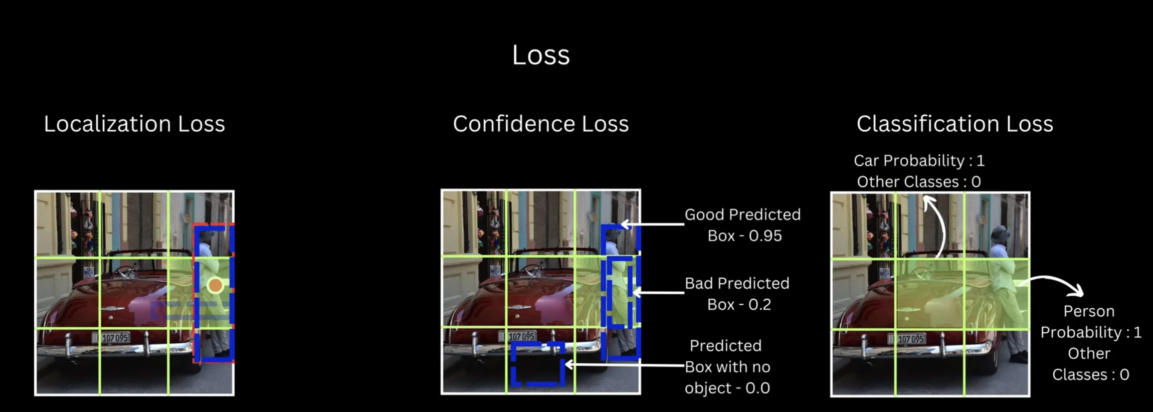 Figure: The three components of YOLO loss function - localization (box coordinates), confidence (objectness), and classification (class probabilities)
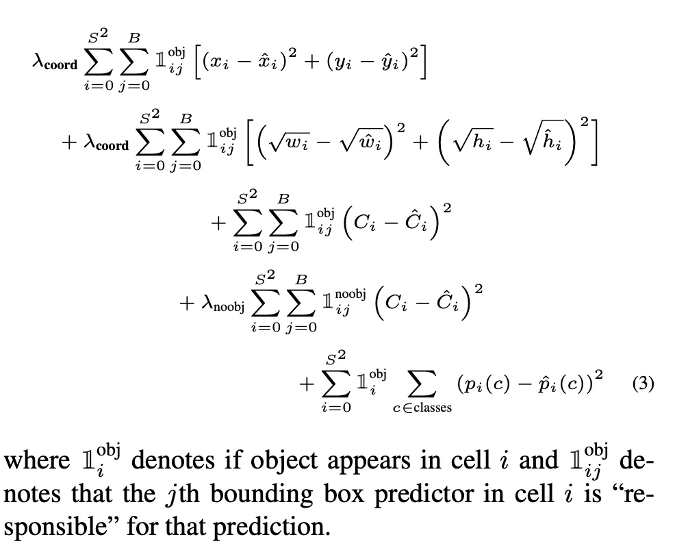 Figure: Detailed breakdown of how each loss component is computed for a single grid cell prediction
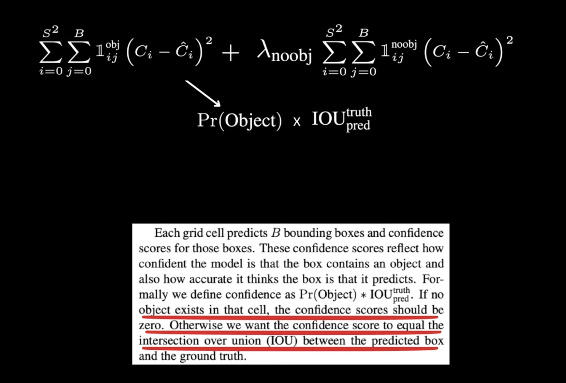 Figure: Classification loss computation showing how class probabilities are compared with one-hot encoded ground truth labels
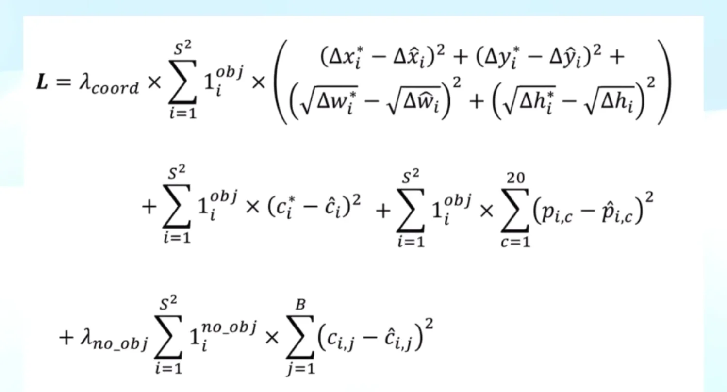 Figure: The complete YOLO loss function combining all three components with their respective weighting factors
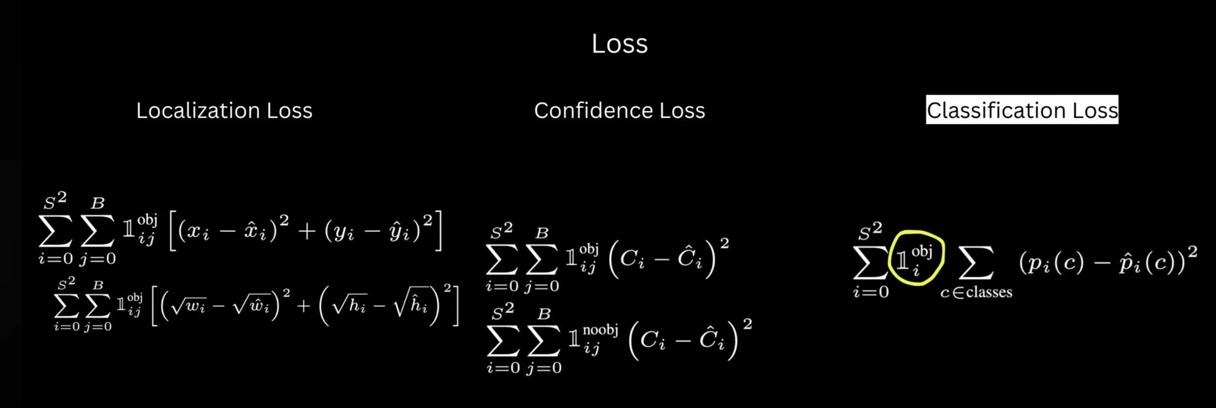 Figure: Mathematical formulation of the complete loss function with indicator functions and summations
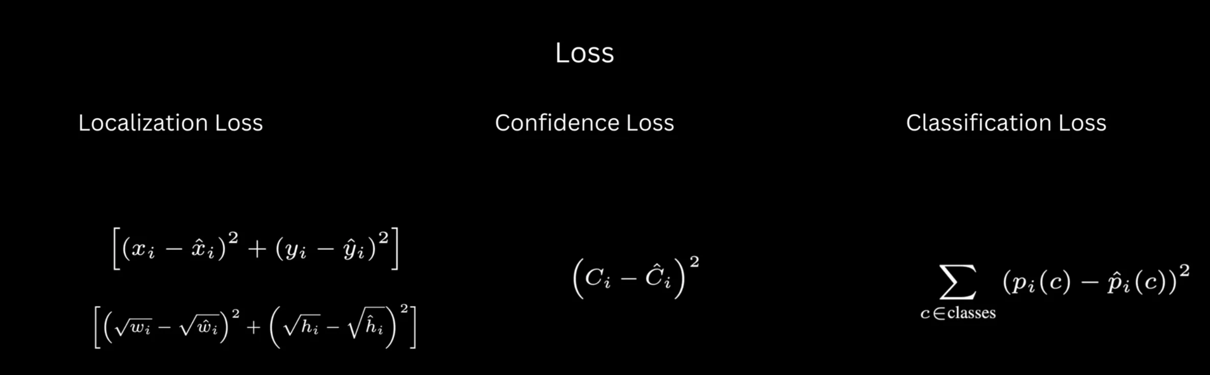 Figure: All three loss components shown together with their mathematical expressions and weighting parameters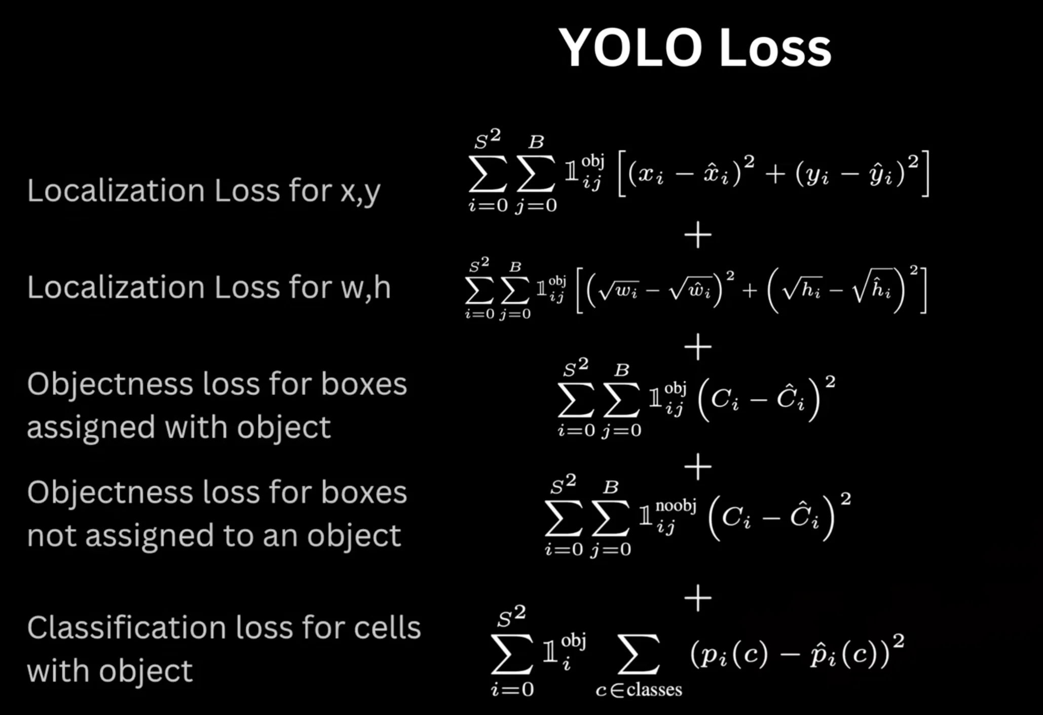
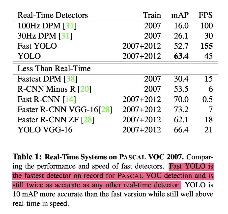 Figure: Performance comparison of YOLOv1 with other detection methods on Pascal VOC 2007 dataset
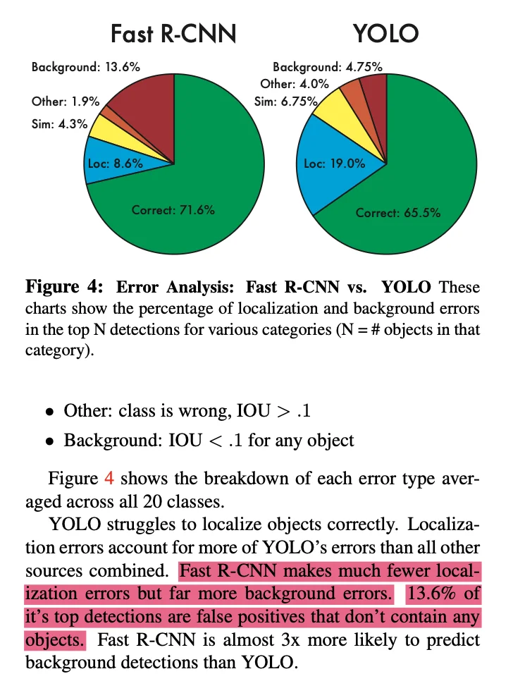 Figure: Detailed accuracy and speed metrics showing YOLO's superiority in real-time performance while maintaining competitive accuracy